Most image segmentation tutorials start with a clean dataset and end with a score. In real projects, a lot of the work happens around that: checking the labels, testing whether a choice like pretraining actually helps, reading the weakest results, and getting the model to run somewhere people can use it.
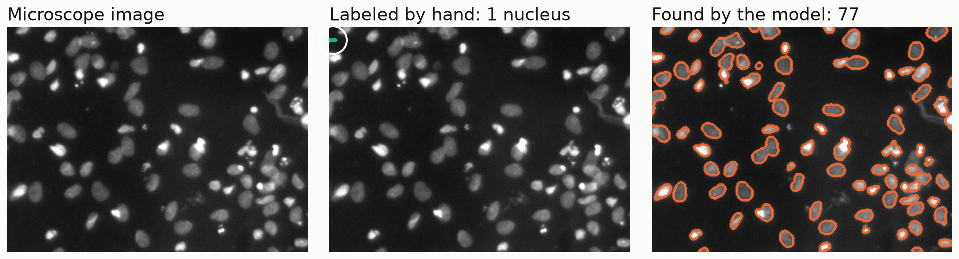
I built a small end-to-end pipeline on public microscopy data to go through each of those steps, with the code and notebook on GitHub. The data is 670 microscope images of cell nuclei, with every nucleus outlined by hand, and the model is a standard U-Net. The part I found most interesting came after training, when I used the model to check the labels it had learned from and found images like the one above.
The data
The images come from the 2018 Data Science Bowl (BBBC038v1 in the Broad Bioimage Benchmark Collection) and are in the public domain. Each image comes with one mask file per nucleus, 29,461 in total. I merged them into one label image per picture, which keeps every nucleus separate for counting later.
The images are not all the same kind. Sorted by color, there are three types:
- Fluorescent (546 images): bright nuclei on a dark background.
- Stained tissue (108 images): purple nuclei in tissue sections.
- Brightfield (16 images): small dark nuclei inside cells, on a light background.
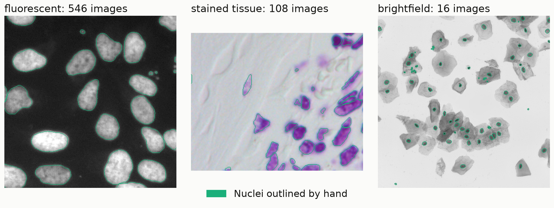
I split the images 70/15/15 into training, validation and test sets, keeping the same mix of types in each part: 470 for training, 100 for validation and 100 for testing. That leaves only 12 brightfield images to train on, which comes back later in the results.
Checking the labels before training
A model learns whatever the masks say, mistakes included. Before any training, I ran a few checks that need only the masks:
| Check | Masks | Images |
|---|---|---|
| A mask broken into separate pieces | 11 | 11 |
| A mask with a hole inside | 425 | 96 |
| A mask over six times the median size in its image (possibly two nuclei) | 34 | 11 |
| Masks overlapping each other | 0 | 0 |
| Near-duplicate image pairs, which would leak between training and test | n/a | 0 |
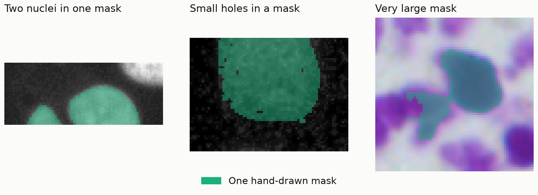
Most holes are tiny, two pixels at the median, so I filled them, since a nucleus has no hole in the middle. The same rule applies to every split, so training and scoring use the same labels. The masks in pieces and the very large masks, 45 masks in 22 images, I left as they were and put on a list for a person to check, because fixing them needs a human eye. No overlaps and no near-duplicates also means the split has no copies across training and test.
I clean the labels before training for two reasons. The first is what the model learns from them: a mask with holes teaches it that parts of a nucleus are background, and a mask that spreads over two objects teaches it to mark the space between them as nucleus. The second is what the scores mean, since the test labels are what the model is measured against. A wrong test label takes points away from a model that is right, a mask in pieces makes the hand count wrong, and a near-copy of a training image in the test set makes the score look better than it is.
Transfer learning, tested rather than assumed
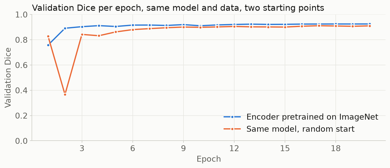
The model is a U-Net with a ResNet34 encoder pretrained on ImageNet, from the segmentation_models_pytorch library. Pretraining on everyday photos usually helps a model learn from a small dataset, but microscope images look very different from ImageNet. So I trained the same model twice with the same data and settings, once from the pretrained weights and once from random weights.
Both runs trained for 20 epochs on random 256 × 256 crops with flips and rotations, with a loss that combines Dice and binary cross-entropy. Each run took about 15 minutes on my laptop with an Apple M-series chip.
| After 1 epoch | After 5 epochs | Best | |
|---|---|---|---|
| Encoder pretrained on ImageNet | 0.758 | 0.905 | 0.925 |
| Same model, random start | 0.828 | 0.862 | 0.911 |
The pretrained model trained more steadily and ended higher, but the gap is small, 0.925 against 0.911. Nuclei are fairly simple shapes, so I was not surprised. On harder images the gap could be much larger, which is why I test it on each new dataset instead of assuming it.
How good is the model?
The score I use is Dice, which measures how well the model's mask overlaps the hand-drawn one. It is the F1 score counted on pixels, where 1 means a perfect match and 0 means no overlap. It leaves out the background, so a model cannot score well by marking nothing, which it could with plain pixel accuracy.
The threshold that turns the model's output into a mask (0.45) was chosen on the validation images only. The test images were scored once, at the end:
| Image type | Test images | Dice | IoU |
|---|---|---|---|
| Fluorescent | 82 | 0.927 | 0.867 |
| Stained tissue | 16 | 0.894 | 0.809 |
| Brightfield | 2 | 0.839 | 0.726 |
| All test images | 100 | 0.920 | 0.855 |
I report the score by image type because an average can hide a type that fails. Brightfield has only two test images, so its number is rough.
To see what the errors look like, I always look at the weakest images:
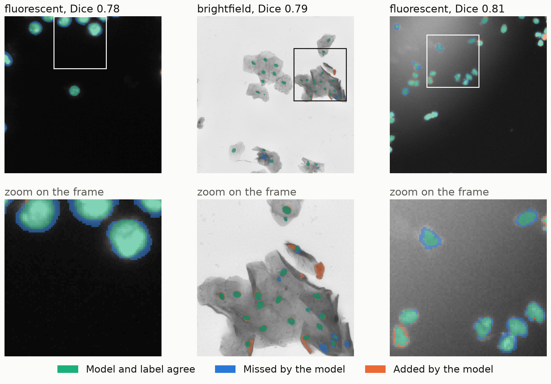
- Fluorescent, Dice 0.78. The model finds all the larger nuclei, but each has a thin blue ring around it. The person who labeled the image included the soft glow around the bright nuclei, and the model draws the edge tighter. It also misses three tiny nuclei. With only 11 small nuclei in the image, these rings are a large share of all nucleus pixels.
- Brightfield, Dice 0.79. This image has real mistakes. The model missed 6 of 46 nuclei in the dark, crowded cell clusters and marked dark folds in the cells as nuclei. Brightfield had only 12 training images.
- Fluorescent, Dice 0.81. Every nucleus is found, again with slightly tighter outlines.
So two of the three weakest images differ from the labels mostly in where exactly the edge is drawn. For counting nuclei that does not matter, but for measuring their size it would, and the fix would be to agree on one rule for where an edge is before labeling more images.
Counting the nuclei
Touching nuclei merge into one blob in a mask, so I split them before counting, with a watershed on the distance to the blob edge. The distance peaks near the center of each nucleus, and each peak grows back out until it meets the edge or a neighbor.
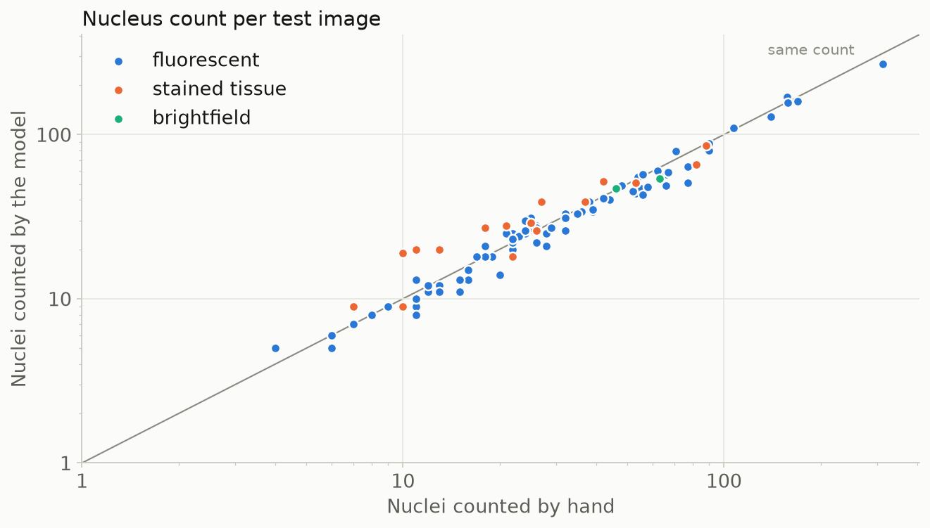
The median count error is 10% on the test images: 9% on fluorescent images and 22% on stained tissue, where the model often counts more nuclei than the person did. Either the splitting step cuts some large tissue nuclei in two, or the labels miss faint nuclei. I would check a sample by eye before changing anything.
What the model found in the labels
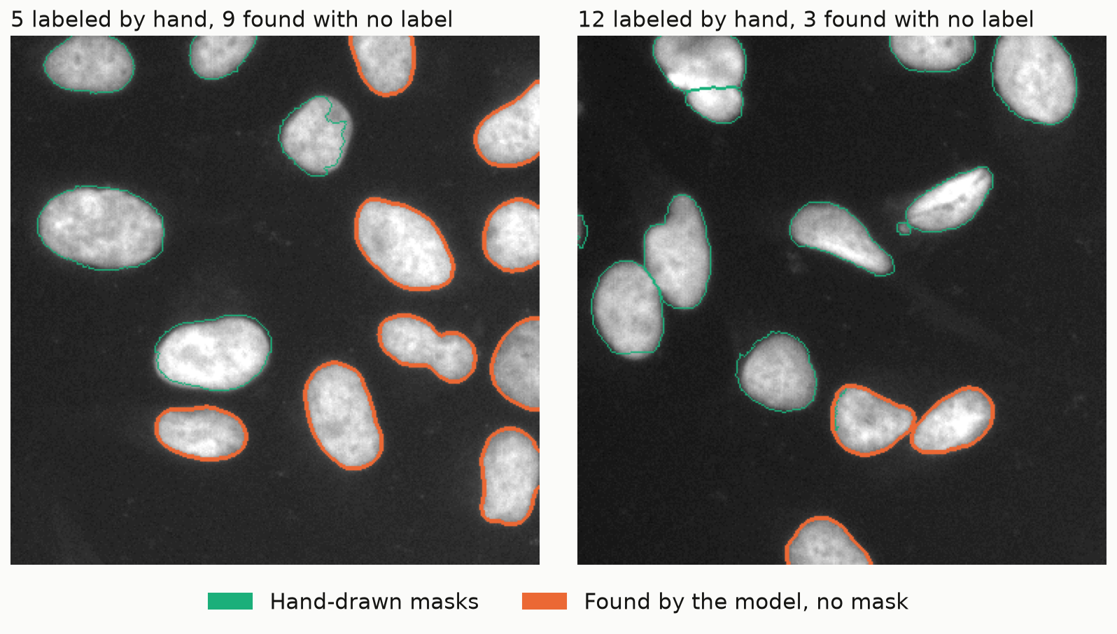
After training, the model can give a second opinion on the labels. For every training and validation image, I compared the nuclei the model found with high confidence against the hand-drawn masks, and listed the ones that have no mask at all. 40 of the 570 images have at least one, 152 nuclei in total.
The image at the top of this post is the clearest case. About 80 nuclei are visible, but only one was labeled by hand, a 26-pixel sliver at the left edge. During training, that image told the model that all the other nuclei were background. The model still found 77 of them, because it learned what a nucleus looks like from the other 469 training images.
There are two things I keep in mind with this check:
- Nobody has checked the 77 one by one. Most are clearly nuclei, but some could be debris, or two touching nuclei inside one outline. That is why the flagged images go to a person for review and nothing is changed automatically.
- The model learned everything from the same hand-drawn labels, and on the test images it still misses edges and faint nuclei. I use it as a second look that points at the images where a label seems wrong, and a person makes the call.
The labels in this dataset are known to contain mistakes, and corrected versions have been published. On a new project, the same check runs on labels that nobody has corrected yet.
Running it on a CPU
A web server usually has no GPU, so I exported the model to ONNX and ran it with ONNX Runtime. The exported model gives the same masks: the largest difference in the raw output was 0.00004, and on the largest test image every pixel got the same decision. I also made an 8-bit version, which uses 8-bit integers instead of 32-bit numbers for the weights and for the values passed between layers, calibrated on 32 training crops.
| Version | File size | CPU time per 512 × 512 image | Test Dice |
|---|---|---|---|
| PyTorch, 32-bit | 98 MB | 199 ms | 0.920 |
| ONNX Runtime, 32-bit | 98 MB | 82 ms | 0.920 |
| ONNX Runtime, 8-bit | 25 MB | 65 ms | 0.917 |
ONNX Runtime ran the model about twice as fast as PyTorch on the same laptop CPU. The timings change a little on every run, so I checked two possible reasons. The speedup held when both were limited to the same four CPU threads, and turning off ONNX Runtime's graph optimizations changed almost nothing. So the gain seems to come from its CPU math routines, which are faster than PyTorch's for this model on this machine. The 8-bit model is four times smaller for a drop in Dice of 0.003, which makes it a good choice for a small server.
A web app and an API
The last step is a small web app built with Gradio. You upload a microscope image, and the app outlines each nucleus and counts them, using the ONNX model on the CPU. The same app also works as an API, so another program can send an image and get the result back. For a platform with its own front end, I also wrapped the model in a plain REST endpoint with FastAPI, which returns the count and the mask.
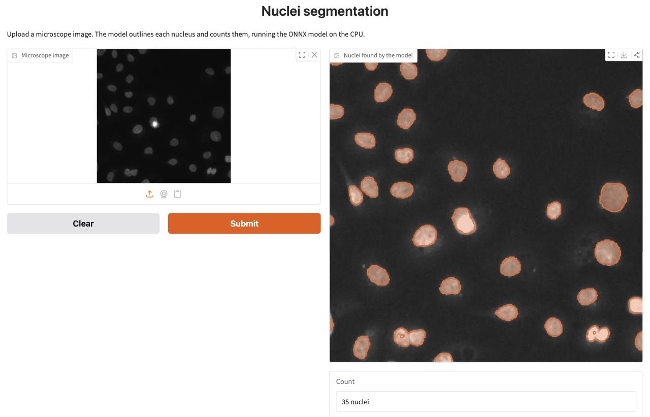
Both run on my laptop. For a real deployment, the next step would be a Docker container on a server, next to the platform that uses the model.
What I would do with real project data
- Split by source (slide, patient or session) instead of by image, so the test score reflects new data rather than more crops of images the model has already seen.
- Run both label checks on the existing labels before training, and agree on a rule for where a nucleus edge is.
- Add more labeled images of the weakest image type before tuning the model.
- Compare two or three architectures on the same split. U-Net, DeepLabV3+ and SegFormer are one line each in the library used here, and I would keep the simplest one that meets the target.
- Serve the 32-bit or the 8-bit ONNX model behind the API, depending on the server.
The notebook, the shared inference code, the REST API and the web app are in the repository on GitHub. Training both models takes about 30 minutes on a laptop with an Apple M-series chip.
Data: Caicedo, J. C. et al. (2019). Nucleus segmentation across imaging experiments: the 2018 Data Science Bowl. Nature Methods 16, 1247-1253. Images and masks are in the public domain (CC0).