When you search for CAM or Grad-CAM online, most tutorials show a heatmap over a photo, usually of a cat or a dog. The setup is always the same: a convolutional neural network (CNN), its last convolutional layer, and a red blob over the part of the image the model relied on.
During my PhD I applied the same two methods, Class Activation Mapping (CAM) and Grad-CAM, to a different kind of input: human pose-estimated skeletons. A skeleton-based model does not see pixels, but rather body keypoints (nodes) connected together forming "bones" (edges), tracked over a few hundred frames (think of it as graph data in time series). The model processes this data with a graph convolutional network (GCN). For this type of data, instead of which region in the image is important, the explanation from an XAI method answers the question which nodes/joints, and when.
The methods carry over almost unchanged, but the details that make them work on graphs are spread across research papers (Pope et al. did it for molecules, Das and Ortega for skeletons), and practical illustrations rarely leave the image domain. This post is that walkthrough: the math with graph indices, PyTorch code, the post-processing skeleton data needs, and the architecture detail that decides whether CAM and Grad-CAM produce the same map.
The running example is EfficientGCN, a spatio-temporal graph convolutional network (ST-GCN) for action recognition on the NTU RGB+D dataset, which I used in a paper in Sensors and in my PhD thesis. Everything else runs in a companion notebook with a small model you can train on a laptop CPU.
The focus here is computing and reading the maps. How faithful and stable they are is a separate question, which the linked papers evaluate.
A short refresher on images
CAM (Zhou et al., 2016) needs a specific structure to the deep learning network. The last convolutional layer produces
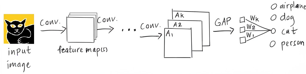
If a feature map has
The weight
Grad-CAM (Selvaraju et al., 2017) removes the architecture requirement. Instead of reading weights from a linear layer, it averages the gradient of the class logit (not the softmax probability, which would change the weights) over each feature map, takes the weighted sum, and keeps the positive part:
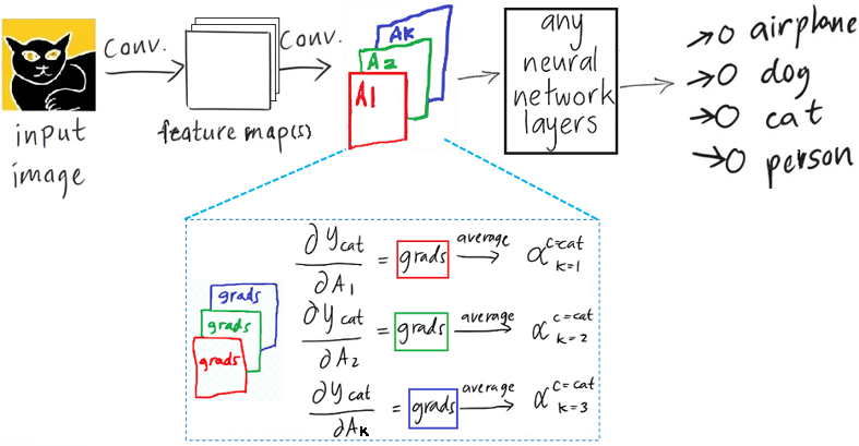
For a more detailed explanation on images, these posts on CAM and Grad-CAM are the best I know.
From pixels to nodes
An NTU RGB+D sample is a skeleton sequence: 25 joints per frame with 3D coordinates, for up to two people. The joints are the nodes of a graph and the bones are its edges. A batch of raw skeletons is a tensor of shape (N, C, T, V, M): samples, coordinate channels, frames, joints and bodies. EfficientGCN's feeder then builds three input branches (joint, velocity and bone) with 6 channels each, so the model itself takes (N, I, C, T, V, M) with I = 3 and C = 6.
The operation that makes the network a graph network is the spatial graph convolution. This is EfficientGCN's, which comes from ST-GCN:
class SpatialGraphConv(nn.Module):
    def forward(self, x):                   # x: (N, C, T, V)
        x = self.gcn(x)                     # 1x1 conv to K groups of channels
        n, kc, t, v = x.size()
        x = x.view(n, self.s_kernel_size, kc // self.s_kernel_size, t, v)
        # A: (K, V, V), one adjacency per hop distance, times learned edge weights
        x = torch.einsum('nkctv,kvw->nctw', (x, self.A * self.edge)).contiguous()
        return x
The einsum mixes each joint's features with its neighbors' along the skeleton. The joint axis goes in as v and comes out as w with the same size: no layer removes a joint. The temporal convolutions in between stride over frames only. So after the whole network, the last feature map of EfficientGCN-B4 still has all 25 joints:
| Image CNN (MobileNetV2) | Skeleton ST-GCN (EfficientGCN-B4) | |
|---|---|---|
| Last feature map | 1280 × 7 × 7 | 272 × 72 × 25 × 2 |
| One position is | one cell of the 7 × 7 grid | one (step, joint, body) index |
| Number of positions |
7 × 7 = 49 | 72 × 25 × 2 = 3,600 |
| Back to the input | upsample 7 × 7 to 224 × 224 | one position per joint, one feature step per 4 input frames |
This is the biggest practical difference from images. A CNN heatmap is blurry because a 7 × 7 grid gets stretched over 224 × 224 pixels. On a skeleton or graph, there is nothing to upsample along the joint axis, so every joint gets its own score. The coarse axis is time, where 288 input frames become 72 feature steps. A position is an index, not a receptive field, though. After many graph layers, plus EfficientGCN's attention over joints and frames, the feature stored at one joint and step can carry information from other joints and many more frames.
CAM on a graph
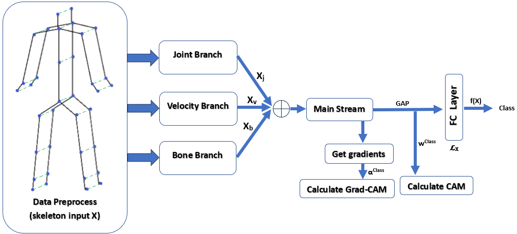
CAM needs GAP followed by one linear layer, and EfficientGCN already ends that way. Its classifier averages over steps, joints and bodies, applies dropout, and finishes with a 1 × 1 × 1 convolution, which is a linear layer written as a convolution:
class EfficientGCN_Classifier(nn.Sequential):
    def __init__(self, curr_channel, num_class, drop_prob, **kwargs):
        super(EfficientGCN_Classifier, self).__init__()
        self.add_module('gap', nn.AdaptiveAvgPool3d(1))
        self.add_module('dropout', nn.Dropout(drop_prob, inplace=True))
        self.add_module('fc', nn.Conv3d(curr_channel, num_class, kernel_size=1))
With graph indices, the only change to the image equations is what a position means. A position is now a (step, joint, body) triple, and
EfficientGCN's forward returns the last feature map next to the logits, so CAM takes one line. The original repository computes it in NumPy for one sample (np.einsum('kc,ctvm->ktvm', weight, feature)). Here is the batched version:
model.eval()                                            # evaluation mode
out, feature = model(x)                                 # feature: (N, C, T, V, M)
weight = model.classifier.fc.weight.flatten(1)          # (num_classes, C)
cam = torch.einsum("kc,nctvm->nktvm", weight, feature)  # (N, num_classes, T, V, M)
For B4 on NTU RGB+D, that is a map of shape (N, 60, 72, 25, 2): a score for every class, step, joint and body, from a single forward pass. If the model is wrapped in DataParallel, the weights are under model.module.classifier.fc.
Grad-CAM on a graph
Grad-CAM uses the same feature map and replaces
EfficientGCN does not include Grad-CAM, so I added it. Because forward returns feature, and feature sits on the path to the logits, PyTorch can differentiate the class score with respect to it directly:
def grad_cam(model, x, target):
    model.eval()  # no dropout, stored BatchNorm statistics
    out, feature = model(x)                          # feature: (N, C, T, V, M)
    score = out.gather(1, target[:, None]).sum()     # each sample's target logit
    grads, = torch.autograd.grad(score, feature)     # same shape as feature
    alpha = grads.mean(dim=(2, 3, 4), keepdim=True)  # average over T, V and M
    return torch.relu((alpha * feature).sum(dim=1))  # (N, T, V, M)
Two notes on this function. My original implementation registered a tensor hook inside forward and called backward() once per sample. Summing the target logits and differentiating once gives the same per-sample gradients, because the classification head processes each sample on its own. That is one backward pass per batch instead of one per sample. model.eval() only switches off dropout and fixes the BatchNorm statistics; gradients still flow. Call the function outside torch.no_grad(), and on the unwrapped model: under multi-GPU DataParallel, the returned feature and logits are gathered separately, so there is no gradient path between them. And if your model does not return its last feature map, capture it with register_forward_hook on the last block.
From a feature map to a skeleton heatmap
Both methods give a map of shape (T, V, M) per sample. Turning it into something you can draw on a skeleton takes four steps, and each one comes from how skeleton datasets are stored:
- Map feature steps to frames. EfficientGCN-B4 reduces the temporal resolution by 4. For display, the original visualizer gives input frame
fthe scores at feature stepf // 4. That is a display convention: each feature can depend on many more than four frames. - Drop the padding. Clips are padded to a fixed length, with zeros in the raw data or by repeating the clip after the usual normalization. The network still produces scores for padded steps. The code below keeps the
length // 4steps whose display frames all lie inside the clip, as my thesis pipeline did. Cropping only cleans up the summary: the padding still influenced the features and the prediction, and - Keep the real body. NTU tensors always have two body slots. For a single-person action the second slot is empty, but it still gets scores. For a two-person action, keep both.
- Keep the positive part, aggregate, then scale. Apply ReLU at every position (Grad-CAM already has), average each joint over the kept steps (the median is more robust to single-step spikes), and divide by the maximum.
def joint_scores(maps, lengths, stride=4, body=0):
    """(N, T, V, M) activation maps -> (N, V) joint scores in [0, 1]."""
    scores = []
    for m, length in zip(maps, lengths):
        steps = max(1, int(length) // stride)           # steps inside the clip
        m = torch.relu(m[:steps, :, body])              # positive part, real body
        s = m.mean(dim=0)                               # or m.median(dim=0).values
        scores.append(s / s.max() if s.max() > 0 else s)
    return torch.stack(scores)
To show every step on something small, the companion notebook trains a four-class model on synthetic skeletons where the motion that defines each class is known. Each class makes one limb move fast (wave right hand, wave left hand, kick right leg, nod head), and every clip also moves a different limb slowly, so the task is to tell the fast target motion from the slow distractor. Clips are 40 to 64 frames long, zero-padded to 64, with an empty second body slot. The model has EfficientGCN's interface and head, and reaches 100% test accuracy after about two minutes of training on a laptop CPU.
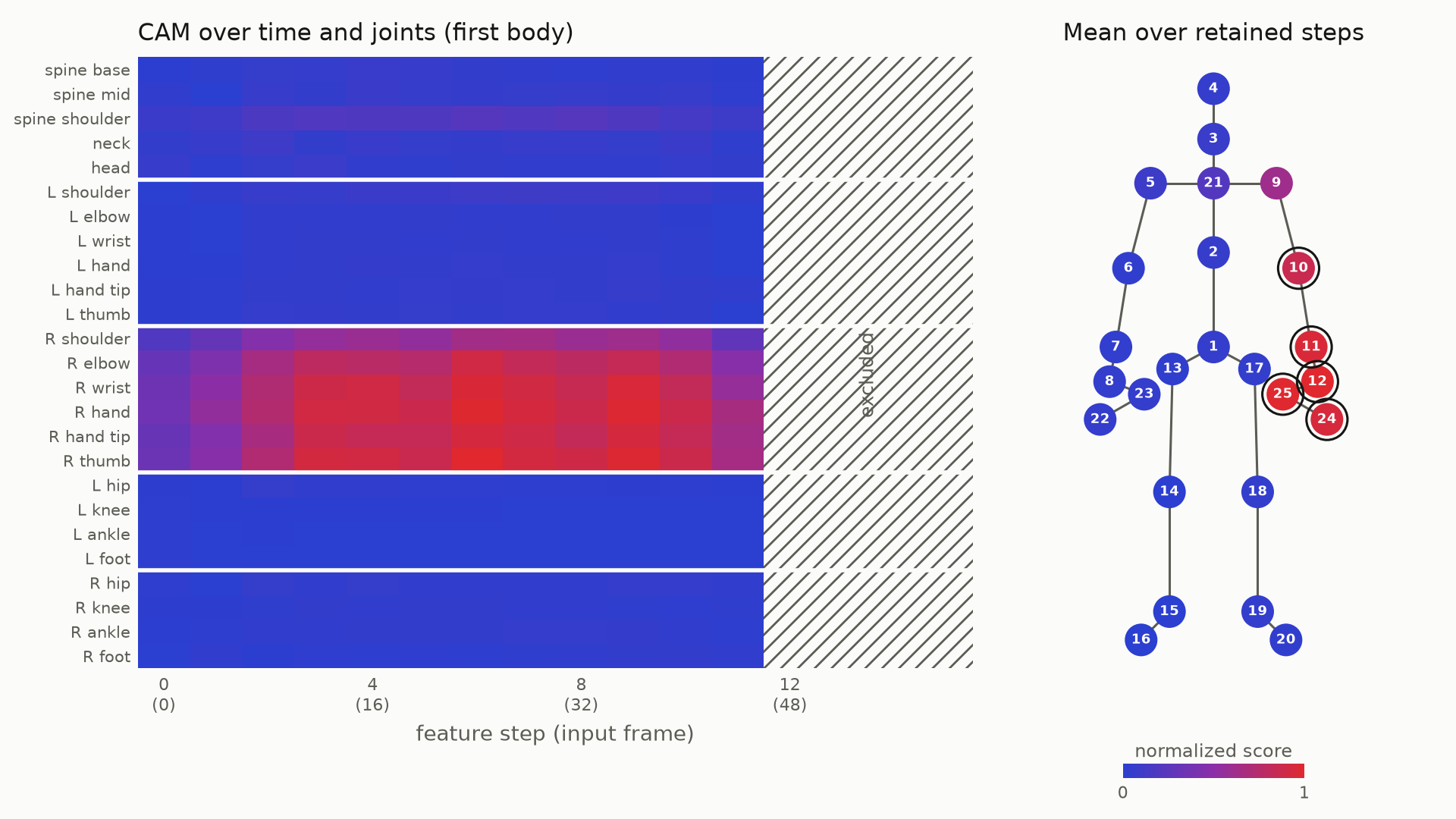
The time axis shows what the averaged skeleton cannot: the right arm's scores are lower in the first and last steps than in the middle of the clip, and the right leg stays blue at every step, even though it moves the whole time.
On real NTU RGB+D data, EfficientGCN-B4's CAM averaged over the frames of a clip looks like this:
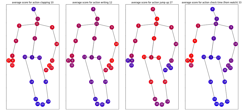
They are easy to read. Clapping lights up both arms and hands. Writing concentrates on the right hand. Jump up moves the evidence to the hips, spine and knees. Check time (from watch) lights up the left forearm and hand, where most people wear a watch. The model was only ever given the action label.
When CAM and Grad-CAM give the same map
In the Sensors paper, CAM and Grad-CAM on EfficientGCN-B4 produced nearly identical explanations. For one standing up sample, the normalized score of the spine base joint was 0.88786113 with CAM and 0.8878651 with Grad-CAM, and the other 24 joints matched just as closely. That is not a coincidence, and it is not specific to skeletons. Follow the gradient through EfficientGCN's head. The class logit is
so the gradient is the same at every position:
Averaging a constant changes nothing, so the Grad-CAM weights are the CAM weights divided by
Grad-CAM is ReLU(CAM) divided by a constant,
N, C, T, V, M = feature.shape
own_cam = cam[torch.arange(N), target]          # (N, T, V, M)
expected = torch.relu(own_cam) / (T * V * M)
torch.allclose(expected, grad_cam(model, x, target))  # True
I ran this on EfficientGCN-B4's own model classes and on the notebook's model, where the largest difference between ReLU(CAM)/
It is the head, not the backbone
That result does not mean CAM and Grad-CAM always agree. Whether they do depends on what sits between the feature map and the class score, and it is easiest to see on images. MobileNetV2 ends in GAP and one linear layer, like EfficientGCN. VGG16 flattens its 7 × 7 map into three linear layers.
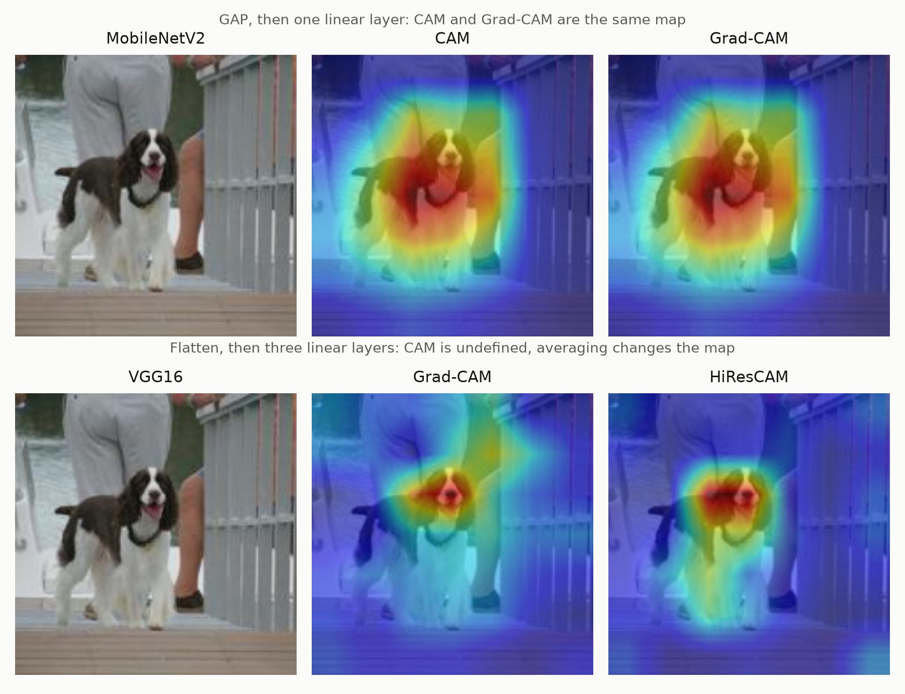
Across the 189 springer spaniel photos that both models classify correctly, MobileNetV2's two maps never differed by more than
On VGG16, CAM is not defined at all. After flattening, each of the 25,088 inputs to the first linear layer has its own weights, so there is no single weight per channel to reuse. You can only get a CAM for VGG16 by changing the model (the CAM paper removes VGG's fully connected layers, adds a convolution, GAP and one linear layer, and fine-tunes), or by borrowing weights that do not belong to channels, which gives a map that is not CAM. If you come across a CAM for VGG16, check which of the two it is.
Grad-CAM still runs on VGG16, but its averaging now throws information away. The gradient differs from position to position, and
On a head like EfficientGCN's, HiResCAM gives the same map as CAM too, because every gradient is
The graph version of VGG16
A graph model can end the same way, for example when the classifier flattens every joint and time step into fully connected layers instead of pooling them, which only works for fixed-size skeletons with a consistent joint order. The notebook trains that variant with the same backbone architecture on the same synthetic data, and it also reaches 100% test accuracy:
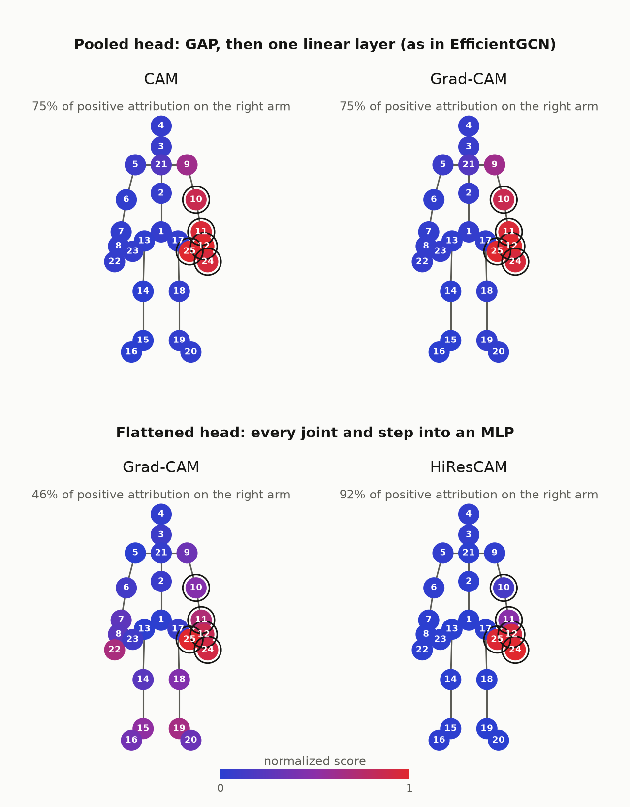
In the run shown here, averaged over the 500 test clips, Grad-CAM put 44% of its positive joint attribution on the target limb and HiResCAM 92%. Equal scores for all 25 joints would put 15% there, since the target limbs have two to five joints. That measures how far the two methods can drift apart, not which one reflects what the network used. The change from Grad-CAM is one line:
return torch.relu((grads * feature).sum(dim=1)) # HiResCAM: no averagingWhether Grad-CAM agrees with CAM or HiResCAM comes down to whether the gradient varies from position to position within a channel. After uniform pooling it cannot, even when an MLP follows, because every position reaches the score through the same pooled value. So the practical rule depends on what follows the explained layer:
| What follows the explained layer | CAM | Grad-CAM |
|---|---|---|
| Mean or sum pooling, then one linear layer | Defined | Same map as CAM, so skip the backward pass |
| Mean pooling, then an MLP | Not defined | Weights depend on the input; same map as HiResCAM |
| Flattened joints and steps, or attention over joints before pooling | Not defined | Can disagree with HiResCAM, because gradients vary by position |
| More graph layers, when you explain an earlier layer such as one input branch | Not defined | Explains that intermediate layer |
Beyond skeletons
Nothing above depends on the graph being a skeleton. Any graph classifier whose last graph layer keeps its nodes and then uses a mean pooling readout and one linear layer supports CAM, whether the nodes are joints, atoms, EEG electrodes or sensors. In PyTorch Geometric, the node-level map is one line:
from torch_geometric.nn import GCNConv, global_mean_pool

class GraphClassifier(torch.nn.Module):
    def __init__(self, in_dim, hidden, num_classes):
        super().__init__()
        self.conv1 = GCNConv(in_dim, hidden)
        self.conv2 = GCNConv(hidden, hidden)
        self.lin = torch.nn.Linear(hidden, num_classes)

    def forward(self, x, edge_index, batch):
        h = self.conv1(x, edge_index).relu()
        h = self.conv2(h, edge_index).relu()              # (num_nodes, hidden)
        return self.lin(global_mean_pool(h, batch)), h

logits, h = model(data.x, data.edge_index, data.batch)
target = logits.argmax(dim=1)                                      # (num_graphs,)
node_cam = (h * model.lin.weight[target][data.batch]).sum(dim=1)  # (num_nodes,)
Graphs in a batch have different numbers of nodes, so each graph's Grad-CAM equals ReLU of its CAM divided by its own node count. Scale scores per graph, not per batch. And if the model uses pooling layers that drop or merge nodes, such as top-k pooling or DiffPool, the last feature map covers the remaining nodes or clusters, and the scores have to be mapped back through those assignments.
What a joint heatmap can and cannot tell you
A few things to keep in mind before reading too much into these maps:
- Scores sit where the evidence ended up. Every graph convolution mixes a joint with its neighbors, and attention like EfficientGCN's pools over all joints and frames, so a joint's features can carry information from elsewhere in the skeleton. In the synthetic clip above, the right shoulder gets no added waving motion, yet CAM gives it a moderate score: it is one bone away from the elbow. Read a bright joint as "the evidence is stored here", not necessarily "the movement happened here".
- Gradient averaging can discard information when gradients vary across positions within a channel, as in the flattened-head example.
- Aggregation is a choice. Mean, median or peak over time can rank joints differently, so say which one you used.
- A heatmap is a hypothesis. Whether the highlighted joints really drive the prediction has to be tested. For these exact methods on skeleton models, my papers in Sensors and IEEE Access evaluate how faithful and stable the explanations are.
Where this matters: early detection of cerebral palsy
The healthcare version of this problem is the reason I started. In the DeepInMotion project at NTNU, an ensemble of spatio-temporal graph networks estimates the risk of cerebral palsy (CP) from videos of infants' spontaneous movements, using 19 tracked body points. CAM and Grad-CAM provide body-point attribution maps for these predictions. For this application, the visualization subtracts the time-aggregated no CP map from the CP map, so joints that score equally for both classes cancel out. The evaluation is in the IEEE Access paper, with code on GitHub.
The full code, including the synthetic data, both models, CAM, Grad-CAM and HiResCAM, the animation at the top of this post, the PyTorch Geometric example, and the MobileNetV2 and VGG16 comparison, is in a notebook on GitHub. The graph parts run on a laptop CPU in a few minutes.
References
- Zhou, B., Khosla, A., Lapedriza, A., Oliva, A. and Torralba, A. (2016). Learning deep features for discriminative localization. CVPR.
- Selvaraju, R. R., Cogswell, M., Das, A., Vedantam, R., Parikh, D. and Batra, D. (2017). Grad-CAM: Visual explanations from deep networks via gradient-based localization. ICCV.
- Draelos, R. L. and Carin, L. (2020). Use HiResCAM instead of Grad-CAM for faithful explanations of convolutional neural networks. arXiv:2011.08891.
- Draelos, R. L. Glass Box Medicine: CNN heat maps: class activation mapping (CAM) and Grad-CAM: visual explanations from deep networks.
- Yan, S., Xiong, Y. and Lin, D. (2018). Spatial temporal graph convolutional networks for skeleton-based action recognition. AAAI.
- Song, Y.-F., Zhang, Z., Shan, C. and Wang, L. (2022). Constructing stronger and faster baselines for skeleton-based action recognition. IEEE TPAMI. Code.
- Shahroudy, A., Liu, J., Ng, T.-T. and Wang, G. (2016). NTU RGB+D: A large scale dataset for 3D human activity analysis. CVPR.
- Pope, P. E., Kolouri, S., Rostami, M., Martin, C. E. and Hoffmann, H. (2019). Explainability methods for graph convolutional neural networks. CVPR. Code.
- Das, P. and Ortega, A. (2022). Gradient-weighted class activation mapping for spatio temporal graph convolutional network. ICASSP. Code.
- Pellano, K. N., Strümke, I. and Ihlen, E. A. F. (2024). From movements to metrics: Evaluating explainable AI methods in skeleton-based human activity recognition. Sensors, 24(6), 1940.
- Pellano, K. N., Strümke, I., Groos, D., Adde, L. and Ihlen, E. A. F. (2025). Evaluating explainable AI methods in deep learning models for early detection of cerebral palsy. IEEE Access, 13, 10126 to 10138.
- Pellano, K. N. (2025). Opening the black box: Explainable spatio-temporal graph convolutional networks for human movement analysis and early cerebral palsy detection. PhD thesis, NTNU.